Neural ODEs and Neural PDEs

Classical data-driven methods in machine learning tend to be data-inefficient and they discard expert modeling knowledge. However, during the last decade a different approach has emerged under the name physics-informed machine learning.

First posted in 2017 and published in 2019, physics-informed neural networks (PINNs) [6] combined deep learning with prior knowledge of the governing equations by directly learning the solution using the PDE residual as a soft penalty in the loss. In 2018, Neural ODEs [1] took a complementary route of embedding the physics in the model itself: the right-hand side of an ordinary differential equation $\dot y=f(y,t)$ is replaced by a neural network $f\approx f_\theta$, trained to reproduce observed data. The same principle was soon extended to stochastic differential equations [7] and to partial differential equations [5] — the latter is what we call here a Neural PDE.

A Neural PDE applies the Neural-ODE construction to an evolution equation in space and time: the unknown coefficient — typically a reaction or source term — becomes a neural network embedded inside a partial differential equation [5], i.e.,

The two constructions are the same idea applied to a finite- and an infinite-dimensional state. The goal of this post is to make that parallel precise within the physics-informed framework. We

1. state both problem formulations in a single notation;
2. define the learning problem (loss, data term, and the regularizer);
3. derive the adjoint equations that give the gradient of the loss; and
4. fit data using explicit Euler for the Neural ODE, and explicit Euler in time with finite elements in space for the Neural PDE.

A brief note on geometric deep learning. Embedding knowledge into the model is one instance of a broader trend. Geometric deep learning [8] pursues the same goal with a different prior: it builds geometric structure — symmetries, invariances, and the shape of the data domain — directly into the architecture. Many successful models are special cases of this principle: convolutional networks encode translation equivariance (1998), graph neural networks respect permutation symmetry (2008), and transformers can be read as attention on a fully connected graph (2017). Where physics-informed learning constrains the model with a governing equation, geometric deep learning constrains it with a symmetry group.

1. Problem formulation

Throughout, $\theta\in\mathbb{R}^p$ denotes the network parameters and $f_\theta$ is a neural network (smooth, e.g. $\tanh$ activations).

1.1 Neural ODE

The state $y(t)\in\mathbb{R}^n$ solves the initial-value problem

with $f_\theta:\mathbb{R}^n\times[0,T]\to\mathbb{R}^n$. We write $y_\theta$ for the solution map $\theta\mapsto y(\,\cdot\,;\theta)$ where we use a discretization scheme such as explicit Euler.

1.2 Neural PDE (Parabolic)

Let $\Omega\subset\mathbb{R}^m$ be a bounded Lipschitz domain with boundary $\Gamma=\partial\Omega$, and let $T>0$ be a finite time horizon. Over the space–time cylinder $\Omega\times(0,T)$ and its lateral boundary $\Gamma\times(0,T)$, the state $y(x,t)$ solves the semilinear parabolic problem

where $\mathcal{A}$ is the second-order elliptic operator in divergence form and $\partial_{\nu_{\mathcal A}}y$ is its associated conormal derivative — the boundary flux that goes with $\mathcal A$, i.e. the outward normal component of the flux $a_{ij}\,\partial_{x_i}y$ that $\mathcal A$ takes the divergence of,

with $(a_{ij})$ symmetric, bounded, and uniformly elliptic, and $\nu$ the outer normal. When $\mathcal A=-\Delta$ we have $a_{ij}=\delta_{ij}$, so the conormal derivative reduces to the ordinary normal derivative $\partial_{\nu_{\mathcal A}}y=\sum_i\partial_{x_i}y\,\nu_i=\nabla y\cdot\nu=\partial_\nu y$ — the most common example. The learnable component is the source term $f_\theta(x,t,y)$ or a boundary term $g_\theta(x,t,y)$.

1.3 Neural PDE (Elliptic)

On the same domain $\Omega$ with boundary $\Gamma=\partial\Omega$, the state $y(x)$ solves the semilinear elliptic problem

with $\mathcal A$ the same divergence-form elliptic operator as before, a nonnegative potential $c_0\in L^\infty(\Omega)$, and a boundary condition of the third kind (Robin) with nonnegative coefficient $\alpha\in L^\infty(\Gamma)$ and datum $g\in L^2(\Gamma)$. As before the learnable component is the source term $f_\theta(x,y)$.

The three problems line up term by term: the finite-dimensional vector field $f_\theta$ stays the learnable right-hand side, the derivative $\dot y$ becomes $\partial_t y$, and the new ingredients are the spatial operator $\mathcal A$ (with a boundary condition) and a fixed reaction $d$. Setting $\partial_t y=0$ then collapses the parabolic problem (PDE-P) onto the elliptic problem (PDE-E), with the reaction $d$ playing the role of the potential $c_0$.

2. The learning problem

We are given data: noisy observations of the true state. We phrase fitting as the minimization of a regularized cost functional $J$. Keeping the general Bolza form lets the same expressions specialize to tracking or terminal objectives.

2.1 Cost functionals

Neural ODE. With a running cost $\varphi$ and terminal cost $\phi$,

Neural PDE (Parabolic). With a distributed cost $\varphi$ on $\Omega\times(0,T)$, a boundary cost $\psi$ on $\Gamma\times(0,T)$, and a terminal cost $\phi$ on $\Omega$,

Neural PDE (Elliptic). With a distributed cost $\varphi$ on $\Omega$ and a boundary cost $\psi$ on $\Gamma$ (no terminal term, since there is no time),

2.2 Data term

Let the data be samples of the true state on a finite set of points,

A least-squares data term is the choice

where $\omega=\sum_{j,k}\delta(x-x_j)\delta(t-t_k)$ is the empirical observation measure (and $\psi=\phi=0$). Concretely the data parts of $J$ read

2.3 Regularization and coercivity

The Tikhonov term $\frac{\gamma}{2}\|\theta\|^2$ is not merely cosmetic — the data term alone need not be coercive in $\theta$ — changes of the parameters can leave the fit almost unchanged, so a minimizing sequence may run off to infinity — and indeed network training problems need not attain an optimum at all [9]. Adding $\frac{\gamma}{2}\|\theta\|^2$ makes the reduced functional coercive,

so sublevel sets are bounded; together with weak lower semicontinuity of $\theta\mapsto J(\theta)$ this yields existence of a minimizer.

3. Adjoint equations

To minimize $J$ we need $\nabla_\theta J$. The adjoint (costate) method, classical in optimal control [2] and PDE-constrained control [4], computes it at the cost of one backward solve, independent of $p=\dim\theta$. We give the continuous adjoint in both settings; the discrete adjoint is what reverse-mode autodiff computes when we differentiate through the integrator, which is why the code can simply call loss.backward().

3.1 Neural ODE adjoint

Introduce the costate $p:[0,T]\to\mathbb{R}^n$ and the Lagrangian

Stationarity with respect to $y$ gives the backward adjoint IVP

and the gradient is

For the data term, $\partial_y\varphi(y_\theta,t)=\sum_k\big(y_\theta(t_k)-y^{\mathrm{obs}}_k\big)\delta(t-t_k)$, i.e. the adjoint receives a jump of size $y_\theta(t_k)-y^{\mathrm{obs}}_k$ at each observation time.

3.2 Neural PDE (Parabolic) adjoint

Let $\mathcal A^{*}$ be the adjoint of $\mathcal A$. Repeating the Lagrangian computation with the weak form of (PDE) and integrating by parts in time (terminal data, since $\delta y(0)=0$) and in space (Green’s identity), the costate $p(x,t)$ solves the backward parabolic problem

where $d_y=\partial_y d$ is the derivative of the known reaction and $\partial_y f_\theta$ that of the learned source — they enter the linearized dynamics as the combined reaction $d-f_\theta$. The gradient is

The structure mirrors (A-ODE) exactly — including the $+$ sign, since $f_\theta$ now sits on the right-hand side just as in (ODE): a backward evolution driven by the cost sensitivity $\varphi_y$, with the adjoint of the linearized dynamics, and a gradient pairing the costate against $\partial_\theta f_\theta$. For the data term, $\varphi_y=\omega\,(y_\theta-y^{\mathrm{obs}})$.

3.3 Neural PDE (Elliptic) adjoint

With no time direction the adjoint is itself a steady elliptic problem. Repeating the Lagrangian computation for the weak form of (PDE-E), the costate $p(x)$ solves

and the gradient is

This is (A-PDE) with the time derivative removed: the same linearized reaction $c_0-\partial_y f_\theta$ and the same conormal-plus-Robin boundary operator, but solved as a single boundary-value problem rather than marched backward in time.

4. Examples with code

The code is in neural-pde/, pure PyTorch. We differentiate through the unrolled integrators with autograd (the discrete adjoint), so the gradients of §3 are obtained without hand-coding the backward solves.

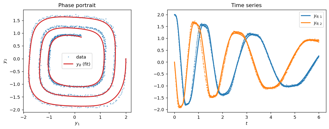
4.1 Neural ODE

Ground truth follows the nonlinear (cubic) spiral example in torchdiffeq [10], $\dot y = A^{\top}y$ with $A=\big[\begin{smallmatrix}-0.1 & 2\\ -2 & -0.1\end{smallmatrix}\big]$ (the cube acting componentwise). We integrate it with explicit Euler, add Gaussian noise to obtain the data $\mathcal D_{\mathrm{ODE}}$, and fit a two–hidden–layer $\tanh$ network $f_\theta$ by minimizing $J_{\mathrm{ODE}}$ with the regularizer of §2.3. The Euler step is

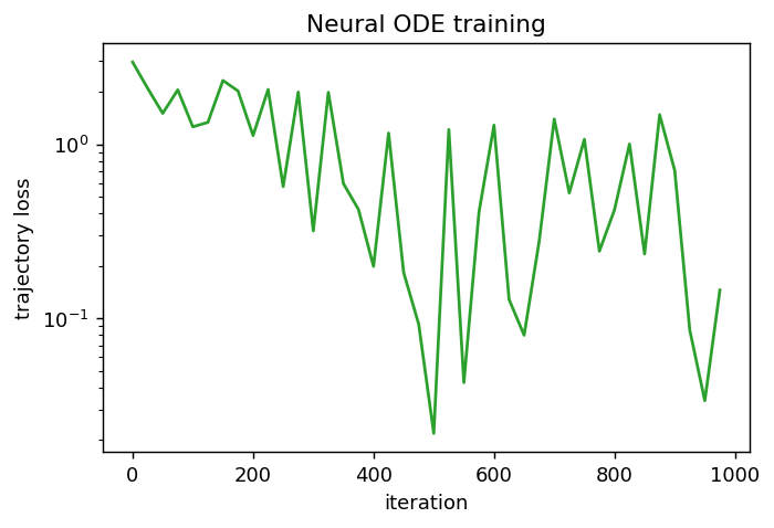
Optimizing one long, full step rollout directly is ill-conditioned, so we use the standard Neural-ODE demo trick [10]: each gradient step is a stochastic estimate of the data term computed from a mini-batch of short sub-trajectories started at points along the data; we keep the checkpoint with the lowest full-trajectory error.

In schematic form, the whole method is the vector field $f_\theta$, the Euler integrator, and a training loop in which loss.backward() is the discrete adjoint of (A-ODE):

class ODEFunc(nn.Module):                       # f_theta: a tanh MLP on R^2
    def __init__(self, dim=2, hidden=64):
        super().__init__()
        self.net = nn.Sequential(
            nn.Linear(dim, hidden), nn.Tanh(),
            nn.Linear(hidden, hidden), nn.Tanh(),
            nn.Linear(hidden, dim))
    def forward(self, y, t):
        return self.net(y)

def euler_rollout(f, y0, t):                     # explicit Euler: y += dt * f(y, t)
    ys, y = [y0], y0
    for k in range(len(t) - 1):
        y = y + (t[k+1] - t[k]) * f(y, t[k])
        ys.append(y)
    return torch.stack(ys)

for it in range(ITERS):                          # minimize J(theta)
    y0_b, t_b, y_target = get_batch()            # short sub-trajectories from data
    y_pred = euler_rollout(func, y0_b, t_b)
    data = 0.5 * ((y_pred - y_target) ** 2).sum(-1).mean()
    reg  = 0.5 * GAMMA * sum((p ** 2).sum() for p in func.parameters())
    opt.zero_grad(); (data + reg).backward(); opt.step()   # discrete adjoint

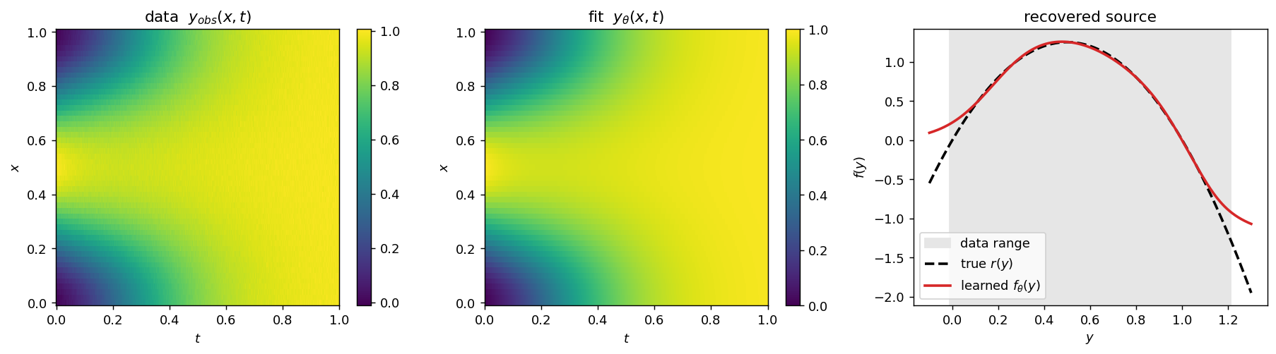
4.2 Neural PDE (Parabolic)

Ground truth is a 1D reaction–diffusion equation on $\Omega=(0,1)$ with homogeneous Neumann (conormal) data, $\mathcal A y=-\nu\,\partial_{xx}y$, known reaction $d\equiv 0$, and source $f_{\mathrm{true}}(y)=5\,y(1-y)$. The state $y(x,t)$ solves

We learn the source $f_\theta(y)$ using a $\tanh$ network acting on nodal values.

Weak formulation. Multiplying by a test function $v\in H^1(\Omega)$, integrating over $\Omega$, and integrating the diffusion term by parts, the boundary term $\nu\,\partial_x y\,v\big|_0^1$ vanishes by the homogeneous Neumann condition. We seek $y(t)\in H^1(\Omega)$ with

which is exactly the form the $P_1$ finite-element discretization below discretizes.

A reaction can only be identified where the data lives, so we simulate several initial conditions; without this coverage the recovered $f_\theta$ is accurate only on the narrow range a single trajectory visits.

Discretization. With $P_1$ finite elements on a uniform mesh we assemble the mass matrix $M$ and stiffness matrix $K$,

and the Neumann condition is natural (no constraint on $K$). Lumping the mass to the diagonal $M_L$, the semidiscrete nodal vector $Y(t)$ obeys

so $L$ is the discrete $\mathcal A$. Marching with explicit Euler (subject to the diffusion stability limit $\Delta t $$ Y^{(k+1)}=Y^{(k)}+\Delta t\,\big(-L\,Y^{(k)}+f_\theta\big(Y^{(k)}\big)\big). $$

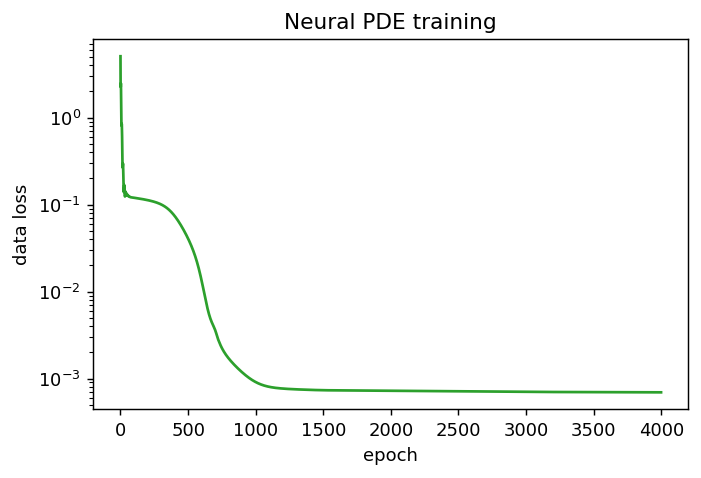
We generate data by simulating $f_{\mathrm{true}}$ from each initial condition, add noise, subsample in time to obtain $\mathcal D_{\mathrm{PDE}}$, and fit $f_\theta$ by minimizing $J_{\mathrm{PDE}}$. The rightmost panel shows that the learned source matches the true nonlinearity across the shaded range of states visited by the data.

The schematic mirrors the Neural-ODE one: the only changes are that the integrator carries the assembled discrete operator $L=\nu M_L^{-1}K$, the state $Y$ is a batch of nodal vectors (one per initial condition), and $f_\theta$ acts pointwise on nodal values:

A_DISC = NU * (1.0 / Mlump)[:, None] * K         # L = nu * M_L^{-1} K  (discrete A)

def fem_euler(source, Y0, t):                    # M_L Y' + nu K Y = M_L f(Y)
    Ys, Y = [Y0], Y0                             # Y0: (n_ic, N_nodes)
    for k in range(len(t) - 1):
        Y = Y + (t[k+1] - t[k]) * (-(Y @ A_DISC.t()) + source(Y))
        Ys.append(Y)
    return torch.stack(Ys)

class Source(nn.Module):                         # f_theta(y), applied at each node
    def __init__(self, hidden=64):
        super().__init__()
        self.net = nn.Sequential(
            nn.Linear(1, hidden), nn.Tanh(),
            nn.Linear(hidden, hidden), nn.Tanh(),
            nn.Linear(hidden, 1))
    def forward(self, Y):
        return self.net(Y.unsqueeze(-1)).squeeze(-1)

for epoch in range(EPOCHS):                      # fit all initial conditions jointly
    Y_pred = fem_euler(model, Y0, t_grid)
    data = 0.5 * ((Y_pred[obs_idx] - Y_obs[obs_idx]) ** 2).sum(-1).mean()
    reg  = 0.5 * GAMMA * sum((p ** 2).sum() for p in model.parameters())
    opt.zero_grad(); (data + reg).backward(); opt.step()

References

[1] Chen, Ricky T. Q., Yulia Rubanova, Jesse Bettencourt, and David K. Duvenaud. “Neural Ordinary Differential Equations.” Advances in Neural Information Processing Systems 31 (2018).

[2] Pontryagin, L. S., V. G. Boltyanskii, R. V. Gamkrelidze, and E. F. Mishchenko. The Mathematical Theory of Optimal Processes. Translated by K. N. Trirogoff, edited by L. W. Neustadt, Interscience Publishers (John Wiley & Sons), 1962.

[3] Tröltzsch, Fredi. Optimal Control of Partial Differential Equations: Theory, Methods and Applications. Graduate Studies in Mathematics 112, American Mathematical Society, 2010. Translated by Jürgen Sprekels. (Semilinear parabolic optimal control: §5.5, problem (5.7)–(5.9), Theorems 5.5 and 5.7, Assumption 5.6. Semilinear elliptic theory: §2.3, §2.5, and §4.2, Theorems 2.7 and 4.4, Assumptions 4.2 and 4.3.)

[4] Lions, Jacques-Louis. Optimal Control of Systems Governed by Partial Differential Equations. Translated by S. K. Mitter. Grundlehren der mathematischen Wissenschaften 170, Springer-Verlag, 1971.

[5] Sirignano, Justin, Jonathan F. MacArt, and Jonathan B. Freund. “DPM: A deep learning PDE augmentation method with application to large-eddy simulation.” Journal of Computational Physics 423 (2020): 109811. https://doi.org/10.1016/j.jcp.2020.109811. (First posted as arXiv:1911.09145 in 2019 under the author order Freund, MacArt, Sirignano.)

[6] Raissi, Maziar, Paris Perdikaris, and George E. Karniadakis. “Physics-informed neural networks: A deep learning framework for solving forward and inverse problems involving nonlinear partial differential equations.” Journal of Computational Physics 378 (2019): 686–707. https://doi.org/10.1016/j.jcp.2018.10.045. (First posted as arXiv:1711.10561, 2017.)

[7] Li, Xuechen, Ting-Kam Leonard Wong, Ricky T. Q. Chen, and David Duvenaud. “Scalable Gradients for Stochastic Differential Equations.” Proceedings of the 23rd International Conference on Artificial Intelligence and Statistics (AISTATS), PMLR 108:3870–3882, 2020.

[8] Bronstein, Michael M., Joan Bruna, Taco Cohen, and Petar Veličković. “Geometric Deep Learning: Grids, Groups, Graphs, Geodesics, and Gauges.” arXiv preprint arXiv:2104.13478, 2021.

[9] Le, Quoc-Tung, Elisa Riccietti, and Rémi Gribonval. “Does a sparse ReLU network training problem always admit an optimum?” Advances in Neural Information Processing Systems 36 (NeurIPS 2023).

[10] Chen, Ricky T. Q. torchdiffeq: differentiable ODE solvers with full GPU support and O(1)-memory backpropagation. GitHub repository, https://github.com/rtqichen/torchdiffeq, example examples/ode_demo.py.

Appendix: well-posedness

For the learning problem of §2 to make sense, the solution map $\theta\mapsto y_\theta$ must be well-defined (and the cost finite) for the parameters explored during training.

A.1 Neural ODE — Picard–Lindelöf

Proposition (existence, uniqueness). Suppose $f_\theta(\cdot,t)$ is measurable in $t$, and there is $L>0$ with

$$|f_\theta(y_1,t)-f_\theta(y_2,t)|\le L\,|y_1-y_2|\quad\forall\,y_1,y_2,\ \text{a.e. }t,$$

together with the linear growth bound $|f_\theta(y,t)|\le C(1+|y|)$. Then for every $y_0\in\mathbb{R}^n$ the problem (ODE) has a unique absolutely continuous solution $y_\theta\in C([0,T];\mathbb{R}^n)$, and $y_\theta$ depends continuously (indeed differentiably) on $\theta$ and $y_0$.

A feed-forward network with globally Lipschitz activations ($\tanh$, ReLU) and bounded weights is globally Lipschitz in $y$ with a constant controlled by the product of the weight-matrix norms, so the hypotheses hold; the growth bound gives existence on the whole of $[0,T]$ (no finite-time blow-up). Differentiable dependence on $\theta$ is what makes $\nabla_\theta J$ in §3.1 meaningful.

A.2 Neural PDE — Tröltzsch’s parabolic theory

Tröltzsch [3], §5.5, studies the semilinear parabolic optimal control problem with a distributed control $v$ and a boundary control $u$,

subject to the state equation

and the control constraints

Our (PDE-P) is exactly the state equation (5.8) with $\mathcal A=-\Delta$ and the right-hand sides taken to be the network $f_\theta$ in the interior and $g$ on the boundary (here $b$ is given). State well-posedness — the solution map being well-defined, which is what §2 needs — is Tröltzsch’s Theorem 5.5.

Theorem 5.5 (Tröltzsch [3]). Suppose that Assumptions 5.1 and 5.4 hold. Then the semilinear parabolic initial–boundary value problem

$$y_t+\mathcal A y+d(x,t,y)=f \ \text{ in } \Omega\times(0,T),\qquad > \partial_{\nu_{\mathcal A}}y+b(x,t,y)=g \ \text{ on } \Gamma\times(0,T),\qquad > y(0)=y_0 \ \text{ in }\Omega$$

has a unique weak solution $y\in W(0,T)\cap C(\overline{\Omega\times(0,T)})$ for any triple $f\in L^r(\Omega\times(0,T))$, $g\in L^s(\Gamma\times(0,T))$, and $y_0\in C(\overline\Omega)$ with $r>N/2+1$ and $s>N+1$. Moreover, there is a constant $c_\infty>0$, which is independent of $d$, $b$, $f$, $g$, and $y_0$, such that

$$\|y\|_{W(0,T)}+\|y\|_{C(\overline{\Omega\times(0,T)})}\le > c_\infty\big(\|f-d(\cdot,0)\|_{L^r(\Omega\times(0,T))}+\|g-b(\cdot,0)\|_{L^s(\Gamma\times(0,T))}+\|y_0\|_{C(\overline\Omega)}\big).\tag{5.6}$$

Assumptions 5.1 and 5.4 are the structural hypotheses on $\mathcal A$, $d$, and $b$ (measurability, boundedness/Lipschitz, and the monotonicity $d_y\ge 0$, $b_y\ge 0$); the integrability thresholds $r>N/2+1$ and $s>N+1$ buy the continuous representative $y\in C(\overline{\Omega\times(0,T)})$. For existence of an optimal solution the problem (5.7)–(5.9) strengthens these to the twice-differentiable Assumption 5.6, which we state together with the existence result verbatim.

Assumption 5.6 (Tröltzsch [3]). (i) $\Omega\subset\mathbb{R}^N$ is a bounded Lipschitz domain.

(ii) The functions

$$d=d(x,t,y):(\Omega\times(0,T))\times\mathbb{R}\to\mathbb{R},\qquad \phi=\phi(x,y):\Omega\times\mathbb{R}\to\mathbb{R},$$

$$\varphi=\varphi(x,t,y,v):(\Omega\times(0,T))\times\mathbb{R}^2\to\mathbb{R},\qquad b=b(x,t,y):(\Gamma\times(0,T))\times\mathbb{R}\to\mathbb{R},$$

$$\psi=\psi(x,t,y,u):(\Gamma\times(0,T))\times\mathbb{R}^2\to\mathbb{R}$$

are measurable with respect to $(x,t)$ for all $y,v,u\in\mathbb{R}$ and, for almost every $(x,t)$ in $\Omega\times(0,T)$ or $\Gamma\times(0,T)$, twice differentiable with respect to $y$, $v$, and $u$. Moreover, they satisfy the boundedness and local Lipschitz conditions (4.24)–(4.25) of order $k=2$; this means that for $\varphi$, for example, there exist some $K>0$ and a constant $L(M)>0$ for any $M>0$ such that, with the objects $\nabla\varphi$ and $\varphi''$ explained in the book,

$$|\varphi(x,t,0,0)|+|\nabla\varphi(x,t,0,0)|+|\varphi''(x,t,0,0)|\le K,$$

$$|\varphi''(x,t,y_1,v_1)-\varphi''(x,t,y_2,v_2)|\le L(M)\big\{|y_1-y_2|+|v_1-v_2|\big\},$$

for almost every $(x,t)\in \Omega\times(0,T)$ and any $y_i,v_i\in[-M,M]$, $i=1,2$.

(iii) We have $d_y(x,t,y)\ge 0$ for almost every $(x,t)\in \Omega\times(0,T)$ and $b_y(x,t,y)\ge 0$ for almost every $(x,t)\in\Gamma\times(0,T)$. Moreover, $y_0\in C(\overline\Omega)$.

(iv) The bounds $u_a,u_b$ and $v_a,v_b:E\to\mathbb{R}$ belong to $L^\infty(E)$ for $E=\Gamma\times(0,T)$ and $E=\Omega\times(0,T)$, respectively, and $u_a(x,t)\le u_b(x,t)$ and $v_a(x,t)\le v_b(x,t)$ for almost every $(x,t)\in E$.

Theorem 5.7 (Tröltzsch [3]). Suppose that Assumption 5.6 holds, and let $\varphi$ and $\psi$ be convex with respect to $v$ and $u$, respectively. Then the optimal control problem (5.7)–(5.9) has at least one optimal pair $(\bar v,\bar u)$ with associated optimal state $\bar y=y(\bar v,\bar u)$.

The monotonicity $d_y\ge 0$, $b_y\ge 0$ in (iii) is the structural condition behind well-posedness of the state equation (5.8). In our learning problem the control is the network $v=f_\theta$, so the relevant nonlinearity is the effective reaction $d-f_\theta$: to stay inside this theory we need $\partial_y(d-f_\theta)\ge 0$ together with the order-$2$ boundedness/Lipschitz bounds — automatic on bounded sets for $\tanh$ networks except for the monotonicity, which one keeps by (i) letting $f_\theta$ depend only on $(x,t)$ (genuine control, $v\in L^\infty(\Omega\times(0,T))$), or (ii) penalizing $\partial_y f_\theta$. Existence of a minimizer in $\theta$ comes instead from the Tikhonov coercivity of §2.3 — the finite-dimensional analogue of the convexity hypothesis on $\varphi,\psi$ in Theorem 5.7. In the example the fixed coercive diffusion $\mathcal A$ dominates on the resolved mesh.

A.3 Neural PDE (Elliptic) — Tröltzsch’s elliptic theory

For the linear problem ($f_\theta=f_\theta(x)$ independent of $y$) Tröltzsch [3], §2.3 and §2.5, gives existence, uniqueness, and an a priori bound for the boundary condition of the third kind.

Theorem 2.7 (Tröltzsch [3]). Let $\Omega\subset\mathbb{R}^N$ be a bounded Lipschitz domain and suppose $c_0\in L^\infty(\Omega)$ and $\alpha\in L^\infty(\Gamma_1)$ satisfy $c_0(x)\ge 0$ and $\alpha(x)\ge 0$ almost everywhere. If one of (i) $|\Gamma_0|>0$ (a Dirichlet part of positive measure), or (ii) $\Gamma_1=\Gamma$ and $\int_\Omega c_0(x)^2\,dx+\int_\Gamma \alpha(x)^2\,ds(x)>0$, holds, then for all $f\in L^2(\Omega)$ and $g\in L^2(\Gamma_1)$ the problem (PDE-E) has a unique weak solution $y\in V$, and there is a constant $c_{\mathcal A}>0$, depending on neither $f$ nor $g$, with

$$\|y\|_{H^1(\Omega)}\le c_{\mathcal A}\big(\|f\|_{L^2(\Omega)}+\|g\|_{L^2(\Gamma_1)}\big).$$

Condition (i) or (ii) excludes the pure-Neumann constant null space (otherwise $y$ is determined only up to a constant): some zeroth-order term — a Dirichlet boundary, the potential $c_0$, or the Robin coefficient $\alpha$ — must pin the solution.

For the semilinear problem the source depends on $y$, and Tröltzsch [3], §4.2, gives well-posedness under the following hypotheses. The boundary value problem is

associated with the bilinear form

Assumption 4.2 (Tröltzsch [3]). (i) $\Omega\subset\mathbb{R}^N$, $N\ge 2$, is a bounded Lipschitz domain with boundary $\Gamma$, and $\mathcal A$ is an elliptic differential operator of the form (2.19) with bounded and measurable coefficient functions $a_{ij}$ that satisfy the symmetry condition and the condition (2.20) of uniform ellipticity.

(ii) The functions $c_0:\Omega\to\mathbb{R}$ and $\alpha:\Gamma\to\mathbb{R}$ are bounded, measurable and almost everywhere nonnegative. At least one of these functions does not vanish almost everywhere, that is, $\|c_0\|_{L^\infty(\Omega)}+\|\alpha\|_{L^\infty(\Gamma)}>0$.

(iii) The functions $d=d(x,y):\Omega\times\mathbb{R}\to\mathbb{R}$ and $b=b(x,y):\Gamma\times\mathbb{R}\to\mathbb{R}$ are bounded and measurable with respect to $x\in\Omega$ and $x\in\Gamma$, respectively, for every fixed $y\in\mathbb{R}$. Moreover, they are continuous and monotone increasing in $y$ for almost every $x\in\Omega$ and $x\in\Gamma$, respectively.

In particular $d(x,0)$ and $b(x,0)$ are then bounded and measurable in $\Omega$ and $\Gamma$.

Assumption 4.3 (Tröltzsch [3]). For almost every $x\in\Omega$ (respectively, $x\in\Gamma$) we have $d(x,0)=0$ (respectively, $b(x,0)=0$). Moreover, $b$ and $d$ are globally bounded, that is, there is a constant $M>0$ such that for any $y\in\mathbb{R}$ we have

$$|b(x,y)|\le M\ \text{ for a.e. } x\in\Gamma,\qquad > |d(x,y)|\le M\ \text{ for a.e. } x\in\Omega.\tag{4.6}$$

Theorem 4.4 (Tröltzsch [3]). Suppose that Assumptions 4.2 and 4.3 hold. Then the elliptic boundary value problem (4.5) has for any pair $f\in L^2(\Omega)$ and $g\in L^2(\Gamma)$ of right-hand sides a unique weak solution $y\in H^1(\Omega)$. Moreover, there is some constant $c_M>0$, which is independent of $d$, $b$, $f$, and $g$, such that

$$\|y\|_{H^1(\Omega)}\le c_M\big(\|f\|_{L^2(\Omega)}+\|g\|_{L^2(\Gamma)}\big).\tag{4.9}$$

The monotonicity of $d$ and $b$ in (iii) is the structural condition behind well-posedness, exactly as in the parabolic case. In our learning problem the source is the network, so the relevant nonlinearity is the effective reaction $d-f_\theta$ (with $d\equiv 0$ in the example): to stay inside this theory we need $\partial_y\big(d-f_\theta\big)\ge 0$, which one keeps by letting $f_\theta$ depend only on $x$ or by penalizing $\partial_y f_\theta$. Existence of a minimizer in $\theta$ again comes from the Tikhonov coercivity of §2.3.