Gaussian Process Regression is one of the most elegant and theoretically rich algorithms in machine learning. With this post, I want to celebrate the mathematical beauty underlying Gaussian Processes. I will divide this post into two sections: theory and practice, accompanied by code examples.
One of the key advantages of Gaussian Processes compared to Deep Learning methods is that they inherently provide interpretability (through confidence intervals and uncertainty estimation). They also offer excellent extrapolation properties, as we will see, and a way to incorporate knowledge about the structure of the data into the model. However, these benefits come at a cost. The algorithm has a wide variety of hyperparameters that are difficult to configure; for instance, kernel selection alone is challenging. Understanding and having a good intuition for the inner workings of this algorithm (and the data) is key to making the most of it.
1. Theory
For context, a Gaussian process is a stochastic process that generalizes the multivariate normal distribution to (potentially) infinite index sets. Wiener studied related objects in 1923 [3], and Krige and others later popularized Gaussian process for regression.
For completeness, here is a standard definition of a Gaussian process:
A process $X(t)$, $t\in I$, is Gaussian if every finite collection $(X(t_1), \dots, X(t_n))$ has a multivariate normal distribution for any $t_1,\dots,t_n\in I$, $n\in\mathbb{N}$.
Consequently, a Gaussian process is fully specified by its mean function $\mu(t)=\mathbb{E}[X(t)]$ and covariance function $\operatorname{Cov}(X(t),X(s)) = \mathbb{E}[(X(t)-\mu(t))(X(s)-\mu(s))]$.
Gaussian processes belong to the family of kernel methods and are studied using the mathematical space: Reproducing Kernel Hilbert Spaces (RKHS). Kernels let us inject prior assumptions about function smoothness, periodicity, linear trends, etc., and often enable powerful nonparametric models with manageable computational cost for modest dataset sizes. Other kernel methods you may know include Kernel PCA (a nonlinear variant of PCA) and Support Vector Machines (SVMs). Even the self-attention can be explained in terms of kernels [4].
Gaussian process regression aims to infer a function $f$ mapping inputs $x$ to outputs $y$, i.e. $y = f(x)$ and we assume that this $f$ is a Gaussian Process with a given covariance. We set up the problem as follows:
- Training inputs: $X=\{x_i\}_{i=1}^n$.
- Latent function values at training inputs: $f = [f(x_1),\dots,f(x_n)]^\top$.
- Likelihood, $p(y|f)$, is Gaussian: $$y_i = f(x_i) + \varepsilon_i \text{, with noise }\varepsilon_i\stackrel{\text{iid}}{\sim}\mathcal N(0,\sigma^2)$$
- Prior on $f(\cdot)\sim \mathcal{GP}$: a Gaussian process with mean $m(\cdot)$ and covariance kernel $k(\cdot,\cdot)$. For now assume $m(\cdot)\equiv 0$; we’ll generalize later.
- Test input: $x_*$ with latent value $f_* = f(x_*)$.
Define covariance matrices/vectors:
- $K \in\mathbb R^{n\times n}$ with $K_{ij}=k(x_i,x_j)$.
- $k_* \in\mathbb R^n$ with $(k_*)_i = k(x_i,x_*) = \operatorname{Cov}(y_i,f_*)$. Note noise on $y$ is independent of $f_*$.
- $k_{**} = k(x_*,x_*) = \operatorname{Var}(f_*)$.
- Covariance of the observed vector $y$: $\mathrm{Cov}(y,y)=K+\sigma^2 I \equiv C_{yy}$.
Some commonly used kernels (covariance functions) in GPR are:
$$ \begin{aligned} k(x,x') &= \exp\left\{-\frac{1}{2\ell^2}\|x-x'\|^2\right\} \quad\text{(Radial Basis Function / RBF)}\\ k(x,x') &= (\gamma x^\top x' + r)^d \quad\text{(Polynomial kernel)}\\ k(x,x') &= \frac{x^\top x'}{\|x\|\cdot \|x'\|} \quad\text{(Cosine similarity kernel)}\\ k(x,x') &= \exp\left\{-\frac{\sin^2\big(\pi|x-x'|/p\big)}{\ell^2}\right\} \quad\text{(Periodic kernel)} \end{aligned} $$In the following sections we will see three different ways to understand the mathematical formulation of GPR.
(Option 1) Best Linear Unbiased Estimator (BLUE)
Our goal is to find the linear estimator $\hat f_* := w^\top y$ that minimizes mean squared error (MSE):
$$ \mathrm{MSE}(w)=\mathbb E\big[(f_* - w^\top y)^2\big]. $$Expand the MSE (expectations are over the joint prior of $f$ and the noise):
$$ \begin{aligned} \mathrm{MSE}(w) &= \mathbb E[f_*^2] - 2\mathbb E[f_* w^\top y] + \mathbb E[w^\top y y^\top w] \\ &= k_{**} - 2 w^\top \mathbb E[y f_*] + w^\top \mathbb E[y y^\top] w. \end{aligned} $$But $\mathbb E[y f_*] = k_*$ and $\mathbb E[yy^\top] = C_{yy} = K + \sigma^2 I$. So
$$ \mathrm{MSE}(w) = k_{**} - 2 w^\top k_* + w^\top C_{yy} w. $$This is a quadratic function of $w$. Differentiate w.r.t. $w$ and set gradient to zero:
$$ \frac{\partial}{\partial w}\mathrm{MSE}(w) = -2 k_* + 2 C_{yy} w = 0 \quad\Rightarrow\quad C_{yy} w^* = k_*. $$Assuming $C_{yy}$ is invertible (typical if $\sigma^2>0$ or $K$ is full rank),
$$ \boxed{w^* = C_{yy}^{-1} k_* = (K+\sigma^2 I)^{-1} k_*.} $$Thus the best linear estimator is
$$ \boxed{\hat f_* = {w^*}^\top y = k_*^\top (K+\sigma^2 I)^{-1} y.} $$This is exactly the usual GP posterior mean (for a zero prior mean).
The minimal MSE (plug $w^*$ back in) is
$$ \begin{aligned} \mathrm{MSE}_{\min} &= k_{**} - {k_*}^\top C_{yy}^{-1} k_*. \end{aligned} $$This equals the GP posterior variance at $x_*$. Thus the minimal achievable MSE by any linear estimator equals the posterior variance.
(Option 2) Orthogonality interpretation
An equivalent derivation uses the orthogonality principle (linear projection): the error $e = f_* - w^\top y$ of the best linear estimator must be uncorrelated with the data used in the estimator:
$$ \mathbb E[e y] = 0 \quad\Rightarrow\quad \mathbb E[(f_* - w^\top y) y] = 0. $$Thus $\mathbb E[f_* y] - \mathbb E[y y^\top] w = 0$, i.e. $k_* - C_{yy} w = 0$, giving the same solution $w = C_{yy}^{-1} k_*$. So the GP predictor is the linear projection of $f_*$ onto the subspace spanned by the observed $y$.
(Option 3) Joint Gaussian conditioning
The standard GP route uses the fact that the joint distribution of $y$ and $f_*$ is Gaussian:
$$\begin{bmatrix} y \\ f_* \end{bmatrix} \sim \mathcal N\left(0, \begin{bmatrix} C_{yy} & k_* \\ k_*^\top & k_{**} \end{bmatrix} \right).$$This follows because any finite collection of evaluations of a Gaussian process is jointly Gaussian. The conditional distribution of a joint Gaussian is
$$ f_* \mid y \sim \mathcal N\big(k_*^\top C_{yy}^{-1} y , k_{**} - k_*^\top C_{yy}^{-1} k_*\big) \tag{Posterior} $$Therefore, the conditional expectation and variance for a multivariate Gaussian yields
$$\mathbb E[f_* \mid y] = k_*^\top C_{yy}^{-1} y, \qquad \operatorname{Var}(f_* \mid y) = k_{**} - k_*^\top C_{yy}^{-1} k_*.$$So the posterior mean equals the linear estimator we derived by minimizing MSE. For Gaussian processes, the posterior mean is both the Bayes (minimum mean squared error over all measurable estimators) and, as we’ve shown, the best linear estimator.
Important conceptual note: for a Gaussian prior the optimal estimator under squared loss is the conditional mean, and because of Gaussianity that conditional mean is linear in $y$. For non-Gaussian priors the best linear estimator (projection) is still $k_*^\top C_{yy}^{-1} y$ but it will not, in general, equal the conditional mean.
1.2 Nonzero mean function
If the GP has mean function $m(\cdot)$, write $m_X = [m(x_1),\dots,m(x_n)]^\top$ and $m_* = m(x_*)$. The model is $y = m_X + (f - m_X) + \varepsilon$. Working with centered quantities $y - m_X$ and $f_* - m_*$ (which have zero mean) gives the estimator
$$ \mathbb E[f_* \mid y] = m_* + k_*^\top (K+\sigma^2 I)^{-1} (y - m_X). $$In practice you subtract the prior mean from the observations, apply the same weight matrix, and add the prior mean back at the test point.
1.3 Complexity analysis
- Training complexity is $\mathcal O(n^3)$ due to the inversion of the the $n\times n$ matrix $C_{yy}$.
- Prediction:
- Mean: $\mathcal O(n)$ per test point after precomputing $C_{yy}^{-1}y$ .
- Covariance: $\mathcal O(n^2)$ per test point if you compute full predictive covariances; computing only marginal variances is cheaper.
For larger datasets, approximate or structured methods (sparse GPs, inducing points, kernel approximations, or GPU-accelerated routines) can improve the speed drastically.
2. Practice and Code
For this implementation we will use the RBF Kernel:
$$ k(x,x') = \exp\left(-\frac{1}{2\ell^2}\|x-x'\|^2\right). $$This kernel is widely used because it is local and universal (see Corollary 4.58 [1]). “Universality” here means the associated RKHS is rich enough to approximate a wide class of continuous functions on compact domains under suitable conditions.
The implementation is straightforward from the previous section.
def rbf_kernel(x1, x2, sigma=1.0):
    y = x1.reshape(-1, 1)-x2.reshape(1,-1)
    return np.exp(-0.5 / sigma**2 * np.square(y))

class GaussianProcess:
    def __init__(self, kernel=rbf_kernel, noise=1e-3):
        self.kernel = kernel
        self.noise = noise

    def fit(self, X_train, y_train):
        self.X_train = X_train
        self.y_train = y_train
        self.K = self.kernel(X_train, X_train) + self.noise * np.eye(len(X_train))
        self.K_inv = np.linalg.inv(self.K)

    def predict(self, X_s):
        K_s = self.kernel(self.X_train, X_s)
        K_ss = self.kernel(X_s, X_s)

        mu_s = K_s.T.dot(self.K_inv).dot(self.y_train)
        cov_s = K_ss - K_s.T.dot(self.K_inv).dot(K_s)
        return mu_s, cov_s
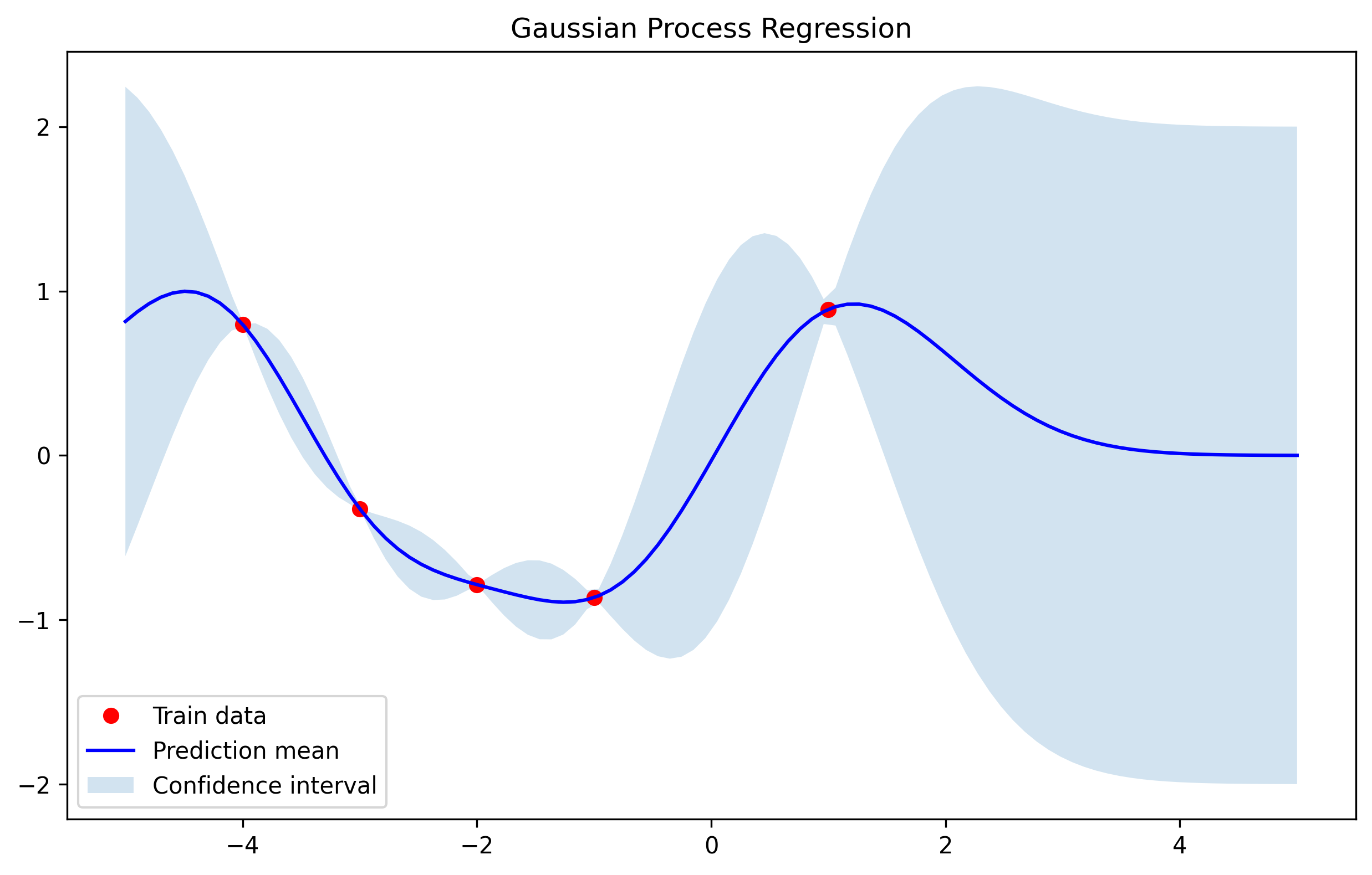
Now we use a very simple dataset, fit the Gaussian Process and plot the results.
# Training data (noisy observations)
X_train = np.array([[-4], [-3], [-2], [-1], [1]]).astype(float)
y_train = np.sin(X_train).ravel() + 0.1 * np.random.randn(X_train.shape[0])

# Test points
X_test = np.linspace(-5, 5, 100).reshape(-1, 1)

# Fit GP and predict
gp = GaussianProcess()
gp.fit(X_train, y_train)
mu_s, cov_s = gp.predict(X_test)
std_s = np.sqrt(np.diag(cov_s))

# Plot
plt.figure(figsize=(10, 6))
plt.plot(X_train, y_train, 'ro', label='Train data')
plt.plot(X_test, mu_s, 'b', label='Prediction mean')
plt.fill_between(X_test.ravel(),
mu_s.ravel() - 2 * std_s,
mu_s.ravel() + 2 * std_s,
alpha=0.2, label='Confidence interval')
plt.legend()
plt.title("Gaussian Process Regression")
plt.show()
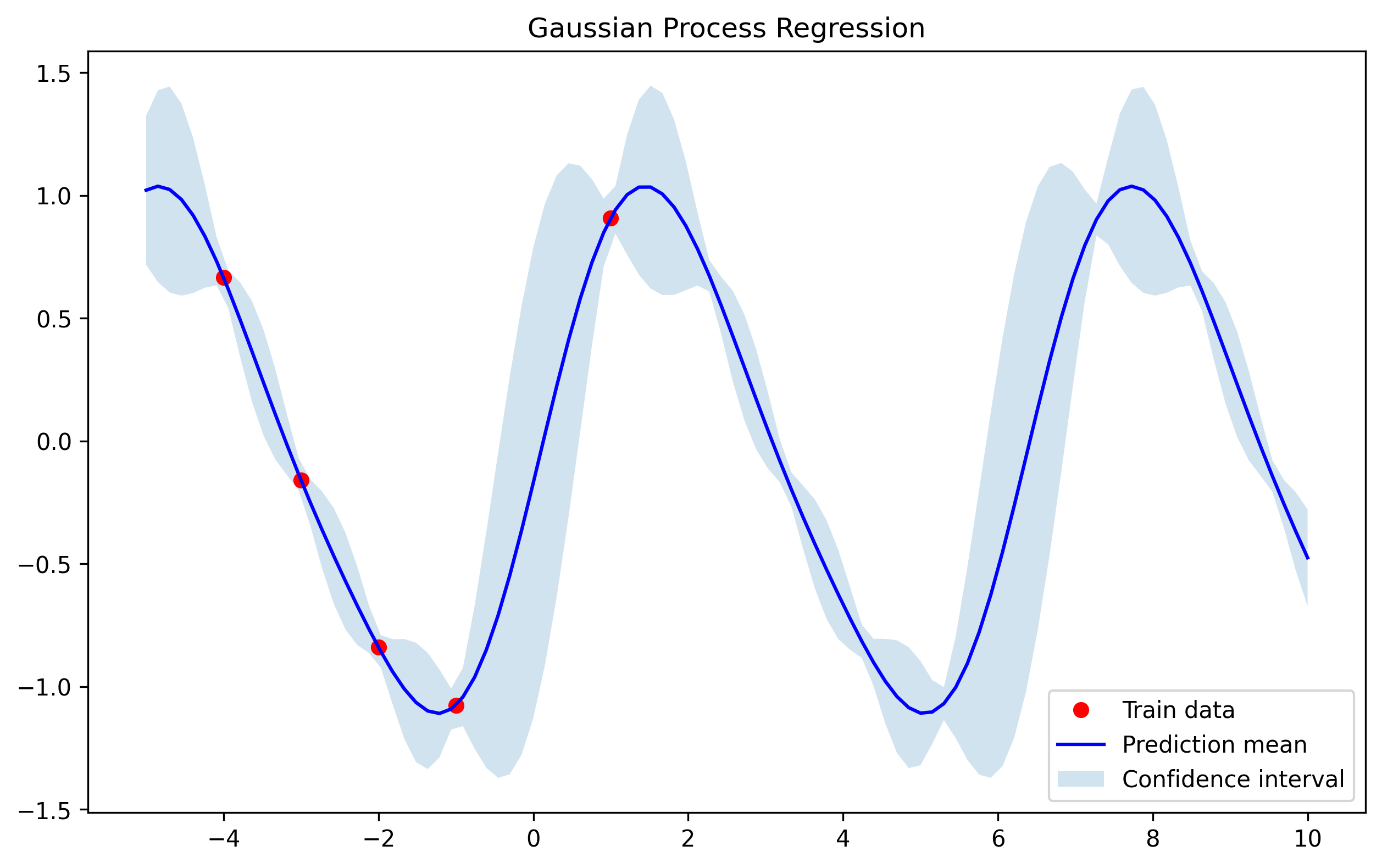
Kernel selection and combination
If the underlying signal is periodic, a periodic kernel is a natural choice. Encoding useful structure in the kernel typically improves extrapolation and predictive performance. For example, the periodic kernel:
def periodic_kernel(x1, x2, period=2*np.pi, l=1.5, sigma=2.0):
    y = x1.reshape(-1, 1) - x2.reshape(1, -1)
    return sigma**2 * np.exp(-2 * (np.sin(np.pi * y / period)**2) / l**2)
Here we are interested in extrapolation outside the data points. Compared to the RBF kernel, a periodic kernel often generalizes better when the signal is truly periodic.
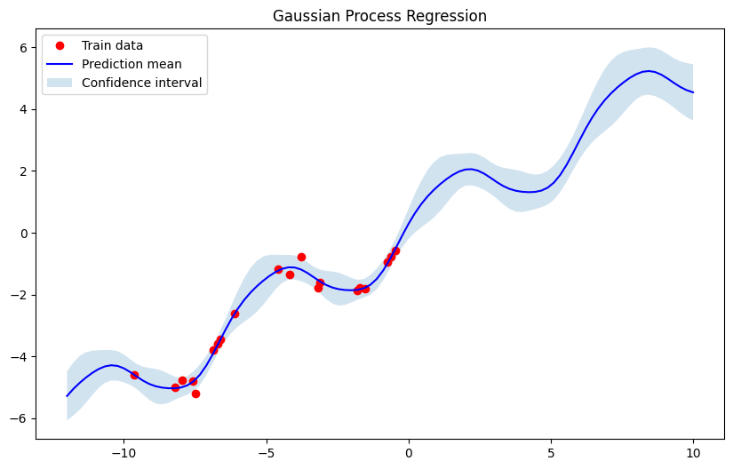
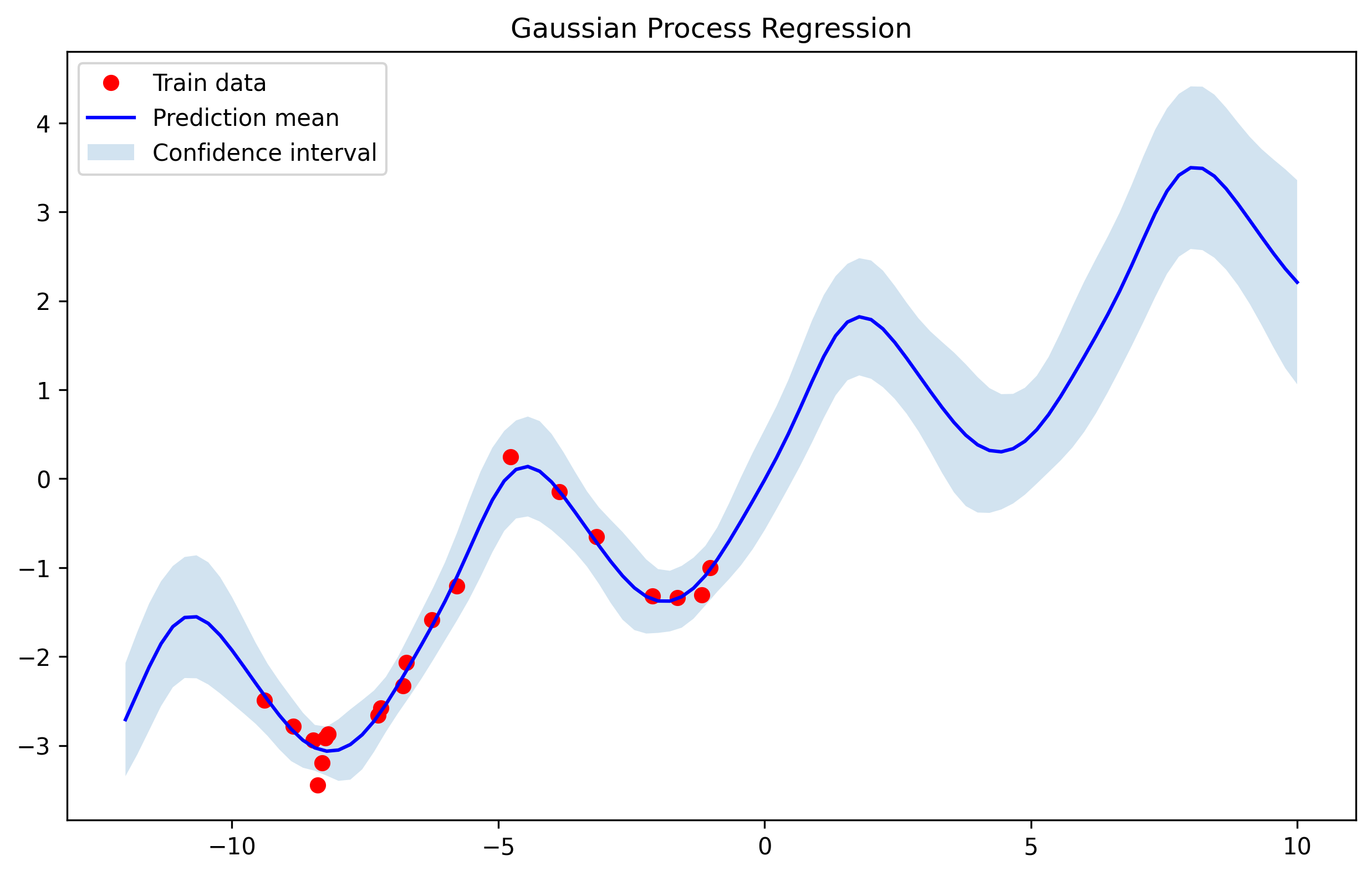
Now, we will explore a more complex example. Assume that our data has a stationary component and also a trend. This problem has been extensively studied in time series and there are already models that can perform this task (see the ARMA family [8]). However, using the Bayesian approach given by Gaussian Processes can lead to similar performance with the added benefit of interpretability.
For this case we will use some of the most interesting properties of kernels:
Kernels can be composed using addition and multiplication.
In this case we are going to combine the periodic kernel with the linear using the sum.
def linear_kernel(x1, x2, c=0.0, sigma=1.0):
    return sigma**2 * (x1.reshape(-1, 1) - c) * (x2.reshape(1, -1) - c)

X_train = (-10 + 20 * np.random.rand(20, 1)).astype(float)
y_train = np.sin(X_train).ravel() + X_train.ravel() / 2 + 0.2 * np.random.randn(20)

# Test points
X_test = np.linspace(-12, 10, 100).reshape(-1, 1)

# Fit GP and predict
addition_kernel = lambda x1, x2: periodic_kernel(x1, x2) + linear_kernel(x1, x2)

gp = GaussianProcess(addition_kernel, noise=0.1)
gp.fit(X_train, y_train)
mu_s, cov_s = gp.predict(X_test)
std_s = np.sqrt(np.diag(cov_s))
And we obtain the following result:
References & Supplementary Material
[1] Steinwart, I. and Christmann, A., 2008. Support vector machines. Springer Science & Business Media.
[2] Williams, Christopher KI, and Carl Edward Rasmussen. Gaussian processes for machine learning. Vol. 2, no. 3. Cambridge, MA: MIT press, 2006.
[3] https://djalil.chafai.net/docs/M2/history-brownian-motion/Wiener%20-%201923.pdf
[4] https://x.com/docmilanfar/status/1974328880564752525
[5] Visual explanation of Gaussian Processes:
https://distill.pub/2019/visual-exploration-gaussian-processes/
[6] Scikit code examples (optimized): https://scikit-learn.org/stable/modules/gaussian_process.html
[7] GPytorch (Efficient GP library using torch as backend): https://github.com/cornellius-gp/gpytorch
[8] Python package for time-series: https://www.statsmodels.org/stable/index.html
Appendix
(A) Gaussian Process Classification
As we saw in section 1, in the case of classification there is no closed form formula to calculate it. In GP classification, the outputs $y_i \in \{0,1\}$, so a Gaussian likelihood doesn’t make sense. Instead, we assume the likelihood is given by a sigmoid function (or logistic):
$$ p(y_i=1 \mid f_i) \equiv \sigma(f_i)= \frac{1}{1 + e^{-f_i}} \tag{Likelihood} $$The joint model is:
$$ p(y, f) = p(y \mid f) p(f) $$where the prior is given by the Gaussian process, as in previous section,
$$ p(f) = \mathcal{N}(f \mid 0, K) \tag{Prior} $$and
$$ p(y \mid f) = \sigma(f)^{y} [1 - \sigma(f)]^{1 - y} $$The problem is that the posterior is intractable. We want:
$$ p(f \mid y) = \frac{p(y \mid f) p(f)}{p(y)} \tag{Posterior} $$but since $p(y \mid f) $ is non-Gaussian, the posterior is not Gaussian and $p(y) = \int p(y \mid f) p(f) df $ is intractable. The solution is to approximate the posterior by a Gaussian distribution. The following table compares both methods.
| Aspect | GP Regression | GP Classification |
|---|---|---|
| Likelihood | Gaussian | Bernoulli via logistic/probit |
| Posterior | Analytic | Approximate (Laplace/EP) |
| Output | Continuous mean, variance | Class probabilities |
| Training | Linear algebra only | Iterative (Newton-Raphson) |
We will use the Laplace approximation to approximate the intractable distribution with a Gaussian centered at its mode.
The idea:
$$p(f \mid y) \approx \mathcal{N}(f \mid \hat{f}, \Sigma)$$where:
- $ \hat{f} = \arg\max_{f} \log p(f \mid \mathbf{y}) $ is the mode,
- $ \Sigma^{-1} = - \nabla^2_{f} \log p(f \mid \mathbf{y}) \big|_{f = \hat{f}} $ is given by the curvature / Hessian at the mode.
Why this makes sense?
The Laplace method relies on a second-order Taylor expansion of the log-posterior around its mode.
(Step 1) Approximate the posterior.
Let:
$$ \psi(f) = \log p(f \mid \mathbf{y}) $$Then we can approximate $\psi(f)$ near its maximum $\hat{f}$ by a quadratic function (the first derivative is zero):
$$ \psi(f) \approx \psi(\hat{f}) - \frac{1}{2} (f - \hat{f})^T A (f - \hat{f}) $$where: $A = - \nabla^2 \psi(f) \big|_{\hat{f}}$. Exponentiating both sides gives:
$$ p(f \mid \mathbf{y}) \propto e^{\psi(f)} \approx e^{\psi(\hat{f})} \exp\left( -\frac{1}{2} (f - \hat{f})^T A (f - \hat{f}) \right) $$That’s just a Gaussian density:
$$ p(f \mid \mathbf{y}) \approx \mathcal{N}(f \mid \hat{f}, A^{-1}) $$Let us apply this to GP classification. We start from the log posterior:
$$ \log p(f \mid \mathbf{y}) = \log p(\mathbf{y} \mid f) + \log p(f) + \text{const} $$Applying log to the (Prior), we obtain
$$ \log p(f) = -\frac{1}{2} f^T K^{-1} f - \frac{1}{2} \log |K| + \text{const} $$And likewise, to the likelihood:
$$ \log p(\mathbf{y} \mid f) = \sum_i \big[ y_i \log \sigma(f_i) + (1 - y_i)\log (1 - \sigma(f_i)) \big] $$(Step 2) Now we will find the mode, denoted by $\hat{f}$.
We maximize $\log p(f \mid \mathbf{y})$ using Newton-Raphson:
$$ \nabla \log p(f \mid \mathbf{y}) = \nabla \log p(\mathbf{y} \mid f) - K^{-1} f $$$$ \nabla^2 \log p(f \mid \mathbf{y}) = -W - K^{-1} $$where
$$ W = -\nabla^2 \log p(\mathbf{y} \mid f) = \text{diag}(\pi_i (1 - \pi_i)), \quad \pi_i = \sigma(f_i) $$We iteratively update:
$$ f_{\text{new}} = f - (K^{-1} + W)^{-1} (\nabla \log p(\mathbf{y} \mid f) - K^{-1} f) $$until convergence to $\hat{f}$.
For a new input $x_*$, the joint prior is:
$$\begin{bmatrix} \mathbf{f} \\ f_* \end{bmatrix} \sim \mathcal{N}\left( 0, \begin{bmatrix} K & k_* \\ k_*^T & k_{**} \end{bmatrix} \right) $$Then, using the joint-conditional argument, the probability of $\mathbf{f}$ under the approximate Gaussian posterior gives:
$$ p(f_* \mid \mathbf{y}) \approx \mathcal{N}(f_* \mid m_*, v_*) $$with:
$$ m_* = k_*^T K^{-1} \hat{\mathbf{f}}, \quad v_* = k_{**} - k_*^T (K^{-1} - K^{-1}\Sigma K^{-1}) k_* $$Then, the predictive class probability is:
$$ p(y_* = 1 \mid \mathbf{y}) = \int \sigma(f_*) p(f_* \mid \mathbf{y}) , df_* \approx \Phi\left( \frac{m_*}{\sqrt{1 + v_*}} \right) $$Now, let us see the results in the code.
class GaussianProcessClassifier:
    def __init__(self, kernel, noise=1e-6):
        self.kernel = kernel
        self.noise = noise

    def fit(self, X_train, y_train, max_iter=100):
        self.X_train = X_train
        self.y_train = y_train.reshape(-1)
        self.K = self.kernel(X_train, X_train) + self.noise * np.eye(len(X_train))

        f = np.zeros_like(self.y_train)

        # Newton-Raphson iteration for Laplace approximation
        for _ in range(max_iter):
            pi = 1 / (1 + np.exp(-f))  # logistic sigmoid
            W = np.diag(pi * (1 - pi))

            B = np.eye(len(X_train)) + np.sqrt(W) @ self.K @ np.sqrt(W)
            B_inv = np.linalg.inv(B)

            sqrt_W = np.sqrt(W)
            b = sqrt_W @ B_inv @ sqrt_W @ self.K @ (self.y_train - pi)

            f = self.K @ b  # update latent f

        self.f = f
        self.W = W
        self.pi = pi
        self.B_inv = B_inv  # store for prediction

    def predict_proba(self, X_s):
        K_s = self.kernel(self.X_train, X_s)
        K_ss = self.kernel(X_s, X_s)

        # Predictive mean and variance for latent function
        sqrt_W = np.sqrt(self.W)
        v = sqrt_W @ K_s
        f_mean = K_s.T.dot(self.y_train - self.pi)
        f_var = np.diag(K_ss - v.T @ self.B_inv @ v)

        # Approximate class probability via probit approximation
        probs = norm.cdf(f_mean / np.sqrt(1 + f_var))
        return probs
And now let us test the result with a dataset that classifies 1 if the data is positive, otherwise it classifies negative.
np.random.seed(42)
X_train = np.linspace(-5, 5, 15).reshape(-1, 1)
y_train = (np.sin(X_train) > 0).astype(int)  # binary labels (0/1)

X_test = np.linspace(-6, 10, 200).reshape(-1, 1)

gp_clf = GaussianProcessClassifier(rbf_kernel)
gp_clf.fit(X_train, y_train)
probs = gp_clf.predict_proba(X_test)
preds = gp_clf.predict(X_test)

# Plot
plt.figure(figsize=(10, 6))
plt.scatter(X_train, y_train, c=y_train, cmap='coolwarm', s=100, edgecolors='k', label='Training data', zorder=3)
plt.plot(X_test, probs[:], 'b-', label='P(y=1)', linewidth=2)
plt.plot(X_test, preds, 'r--', label='Predictions', linewidth=2, alpha=0.7)
plt.xlabel('X', fontsize=12)
plt.ylabel('Value', fontsize=12)
plt.legend()
plt.grid(alpha=0.3)
plt.title('Gaussian Process Classification')
plt.tight_layout()
plt.show()
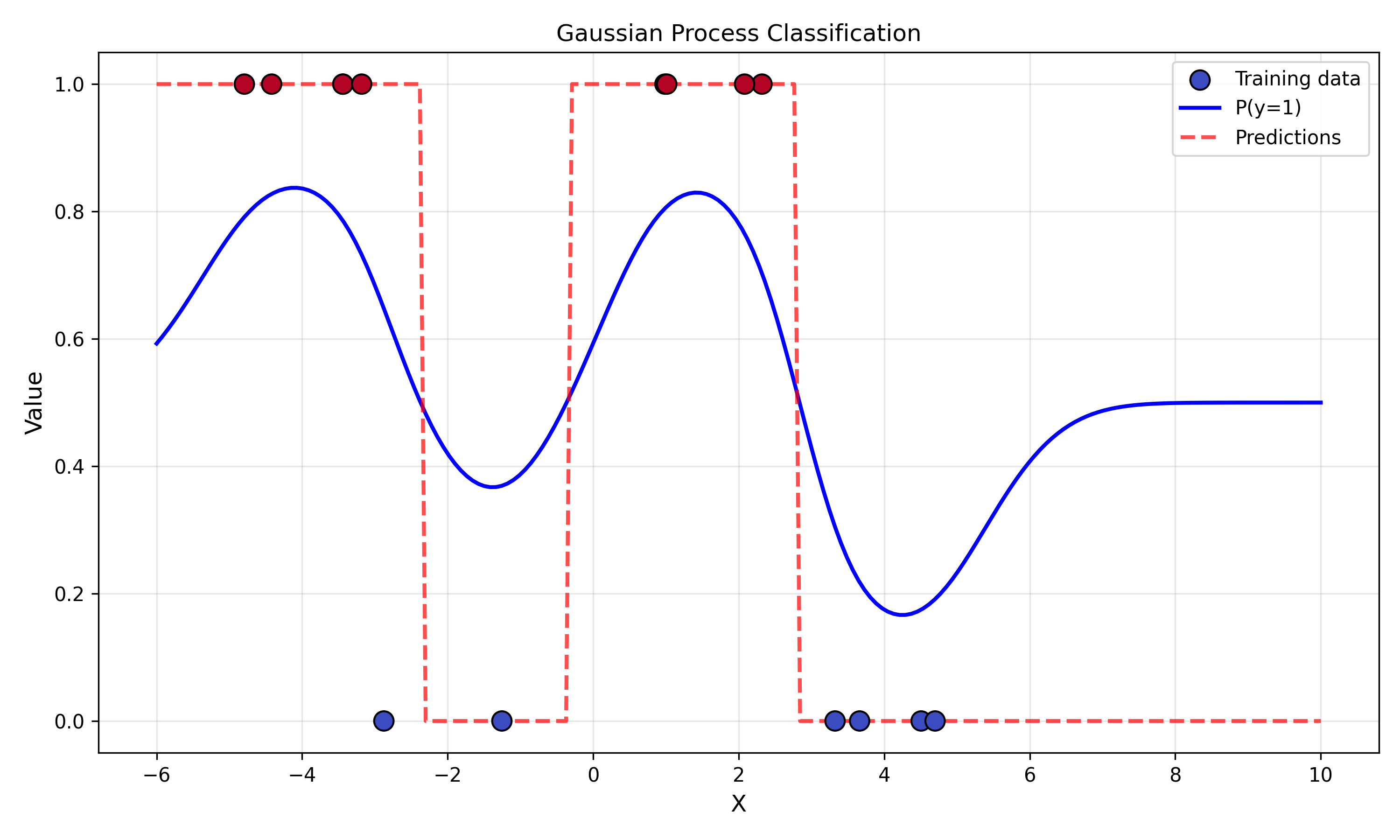
Note: in this example a periodic kernel would be more appropriate than a plain RBF kernel. I leave trying that variant as an exercise to the reader heheheh.
(B) Functional Gaussian Processes
So far, inputs have been finite-dimensional vectors. The extension to the Euclidean space ($x\in\mathbb{R}^n$, $y\in\mathbb{R}^m$) is straightforward. But we can go further:
What if each input is itself a function?
This question lies at the heart of Functional Data Analysis (FDA). We can define kernels on function spaces and apply GP machinery to map functions to scalars or to other functions. For simplicity we focus on scalar outputs $y\in\mathbb{R}$.
For example, suppose inputs are Brownian-motion trajectories and the goal is to predict the endpoint $x(T)$ given the trajectory on [0,T]. One can use a functional RBF kernel based on the L^2 distance between functions:
$$ k(x,x') = \exp\left(-\frac{1}{2\sigma^2}\|x-x'\|_{L^2}^2\right) \tag{Functional RBF} $$and proceed with the standard GP workflow. Example code follows.
def rbf_kernel(x1, x2, dt, sigma=1.0):
    y = np.square(x1[:, None, :] - x2[None, :, :])
    integral = np.sum(dt * (y[...,:-1] + y[...,1:]) * 0.5, axis=-1)
    return np.exp(-1 / (2*sigma**2) * integral)
Generate the dataset and use the Gaussian Process to fit and predict. Notice that we use the same GaussianProcess class as before.
N = 100
num = 10
dt = 1/(N-1)
t = np.linspace(0,1,N)

def generate_brownian(num, N):
    incs = np.sqrt(dt) * np.random.randn(num, N-1)
    return np.concatenate((np.zeros((num,1)), np.cumsum(incs, axis=1)), axis=1)

X_train = generate_brownian(num, N)
X_test = generate_brownian(3, N)

# Training data (noisy observations)
y_train = X_train[:,-1] + 0.1 * np.random.randn(X_train.shape[0])
y_test = X_test[:,-1]

# Fit GP and predict
gp = GaussianProcess(rbf_kernel, dt)
gp.fit(X_train, y_train)
mu_s, cov_s = gp.predict(X_test)
std_s = np.sqrt(np.diag(cov_s))
We obtain the following results for the the 3 test samples.
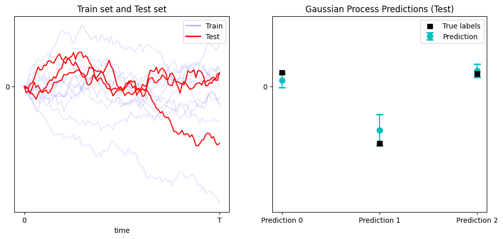
The results are quite good despite only using 10 training samples.
(C) Stable Gaussian Process with Cholesky decomposition
One practical aspect we have skipped is numerical stability when inverting $C_{yy}$. Direct inversion is not recommended. A better approach is to use the Cholesky decomposition. Note that $C_{yy} = K + \sigma^2 I$ is positive definite when $\sigma^2>0$ (since $K$ is positive semi-definite). Hence we can write
$$ C_{yy} = L L^\top $$(1) Predictive mean:
$$ \mathbb{E}[f_* \mid y] = k_*^\top C_{yy}^{-1} y $$Instead of computing $C_{yy}^{-1}$, we solve the equivalent linear system using the Cholesky factors:
- Solve $L v = y$
- Solve $L^\top \alpha = v$
Now $\alpha = C_{yy}^{-1} y$. So the mean is:
$$ \mathbb E[f_* \mid y] = k_*^\top \alpha $$(2) Predictive covariance
The predictive covariance is:
$$ \operatorname{Var}(f_* \mid y) = k_{**} - k_*^\top C_{yy}^{-1} k_* $$Again, avoid $C_{yy}^{-1}$. Instead compute:
- Solve $L v = k_*$.
- Then $k_*^\top C_{yy}^{-1} k_* = v^\top v$.
So:
$$ \operatorname{Var}(f_* \mid y) = k_{**} - v^\top v $$The result looks as follows
class GaussianProcess:
    def __init__(self, kernel, noise=1e-3):
        self.kernel = kernel
        self.noise = noise

    def fit(self, X_train, y_train):
        self.X_train = X_train
        self.y_train = y_train
        K = self.kernel(X_train, X_train) + self.noise * np.eye(len(X_train))
        self.L = np.linalg.cholesky(K)

    def predict(self, X_s):
        K_s = self.kernel(self.X_train, X_s)
        K_ss = self.kernel(X_s, X_s)

        v = np.linalg.solve(self.L, self.y_train) # First solve L v = y
        alpha = np.linalg.solve(self.L.T, v) # Then solve L^T alpha = v
        mu_s = K_s.T.dot(alpha)

        v = np.linalg.solve(self.L, K_s) # Solve for L\K_s
        cov_s = K_ss - v.T.dot(v)

        return mu_s, cov_s
(D) Relation between Gaussian Process Regression and Maximum Mean Discrepancy (MMD)
Let $\mathcal H$ be the RKHS with reproducing kernel $k(\cdot,\cdot)$. For a location $x$ denote the representer $k_x := k(\cdot,x)\in\mathcal H$. For two (signed) measures $\mu,\nu$ the squared MMD (kernel mean embedding distance) is
$$ \mathrm{MMD}^2(\mu,\nu) = \|\mu-\nu\|_{\mathcal H}^2 = \| m_\mu - m_\nu\|_{\mathcal H}^2, $$where $m_\mu=\int k(\cdot,x),d\mu(x)$ is the kernel mean map. For discrete/signed measures this reduces to kernel sums.
Take the target distribution $\mu=\delta_{x_*}$ (a unit mass at the test point) so $m_\mu = k_{x_*}$. Take a weighted empirical signed measure $\nu_w=\sum_{i=1}^n w_i \delta_{x_i}$ so $m_{\nu_w}=\sum_i w_i k_{x_i}$. Then
$$ \mathrm{MMD}^2\big(\delta_{x_*},\nu_w\big) = \|k_{x_*} - \sum_{i} w_i k_{x_i}\|_{\mathcal H}^2. $$Use reproducing-kernel identities to expand that squared RKHS norm:
$$ \begin{aligned} \|k_{x_*} - \sum_i w_i k_{x_i}\|_{\mathcal H}^2 &= \langle k_{x_*},k_{x_*}\rangle - 2\sum_i w_i\langle k_{x_*},k_{x_i}\rangle \sum_{i,j} w_i w_j \langle k_{x_i},k_{x_j}\rangle \\ &= k_{**} - 2 w^\top k_* + w^\top K w. \end{aligned} $$This is the MMD between $\delta_{x_*}$ and the weighted empirical measure $\nu_w$.
Relation to the MSE quadratic form
Recall from the linear-estimation derivation (zero-mean case) that the MSE of the linear estimator $\hat f_* = w^\top y$ equals
$$ \mathrm{MSE}(w) = \mathbb E\big[(f_* - w^\top y)^2\big] = k_{**} - 2 w^\top k_* + w^\top (K + \sigma^2 I) w. $$Compare this with the MMD expansion above: the difference is exactly the noise term $\sigma^2 w^\top w = \sigma^2 \|w\|_2^2$. Thus we can write
$$ \boxed{\mathrm{MSE}(w) = \underbrace{\mathrm{MMD}^2 (\delta_{x_*},\nu_w )}_{\text{deterministic RKHS discrepancy}}+ \sigma^2 \|w\|_2^2.} $$So minimizing mean-squared error over linear estimators is equivalent to choosing weights $w$ that minimize the RKHS discrepancy (MMD) between the target at $x_*$ and the weighted training points, regularized by the squared $\ell_2$-norm of the weights weighted by the noise variance.