Feynman–Kac formula

There is a beautiful connection between probability theory and partial differential equations (PDEs), given by the famous Feynman–Kac theorem.

This result allows us to translate between stochastic finite-dimensional problems and deterministic infinite-dimensional problems. It appears everywhere in finance, physics, control theory, and machine learning (generative modeling and reinforcement learning).

What makes this connection especially useful is that it works in both directions.

A high-dimensional PDE (very expensive to solve numerically) can be evaluated at a single point simply by simulating a random process. Conversely, a difficult question about a stochastic process can be transformed into a deterministic PDE and tackled using standard techniques.

Example. Take the Dirichlet problem

$$ \begin{cases} \Delta u = 0 & \text{in } \Omega, \\ u = g & \text{on } \partial\Omega. \end{cases} $$

The Feynman–Kac theorem says its solution is

$$ u(x) \;=\; \mathbb{E}\big[\,g(B_\tau)\,\big] $$

where $B$ is a Brownian motion started at $x$ and $\tau$ is the first time it leaves $\Omega$.

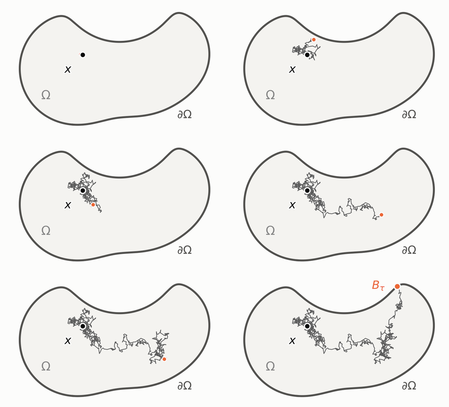
The proof is short, and worth seeing once before the general statement. It needs one tool, the chain rule for Brownian paths.

Itô’s formula. For $\varphi\in C^2(\mathbb{R}^d)$ and a Brownian motion $B$,

$$ d\varphi(B_t) \;=\; \nabla\varphi(B_t)^\top dB_t \;+\; \tfrac12\Delta\varphi(B_t)\,dt . $$

The second term is what an ordinary chain rule misses. The path is nowhere differentiable, but it accumulates quadratic variation at a definite rate, $d\langle B^i,B^j\rangle_t=\delta_{ij}\,dt$, and the Laplacian is what that second-order term collects.

Proof of the example. Let $\Omega$ be bounded, let $u\in C^2(\Omega)\cap C(\overline\Omega)$ solve the problem, let $B$ start at $x\in\Omega$ and let $\tau=\inf\{t>0:\;B_t\notin\Omega\}$.

Check first that the path leaves at all. Itô’s formula on $h(y)=|y|^2$, for which $\tfrac12\Delta h=d$, gives $\mathbb{E}_x\big[|B_{t\wedge\tau}|^2\big]-|x|^2=d\,\mathbb{E}_x[t\wedge\tau]$, whose left-hand side is at most $\sup_{y\in\overline\Omega}|y|^2$; letting $t\to\infty$ and using monotone convergence, $\mathbb{E}_x[\tau]<\infty$, and in particular $\tau<\infty$ almost surely.

Now Itô’s formula applied to $u$ leaves

$$ du(B_t) \;=\; \nabla u(B_t)^\top dB_t , $$

the $dt$ term vanishing because $u$ is harmonic. So the stopped process $M_t:=u(B_{t\wedge\tau})$ is a local martingale, and it is bounded by $\sup_{\overline\Omega}|u|$; hence it is a martingale and

$$ u(x) \;=\; \mathbb{E}_x\big[\,u(B_{t\wedge\tau})\,\big] \qquad\text{for every } t . $$

Letting $t\to\infty$, $u(B_{t\wedge\tau})\to u(B_\tau)=g(B_\tau)$ because the path does exit and $u$ is continuous up to the boundary, and bounded convergence turns the display into

$$ u(x) \;=\; \mathbb{E}_x\big[\,g(B_\tau)\,\big]. \qquad\blacksquare $$

1. The Feynman–Kac theorem

Let $X$ solve the SDE

$$ dX_t \;=\; b(X_t)\,dt + \sigma(X_t)\,dW_t $$

in $\mathbb{R}^d$, with $b,\sigma$ Lipschitz.

Theorem (Feynman–Kac). Let $V,g:\mathbb{R}^d\to\mathbb{R}$ and $f:[0,T]\times\mathbb{R}^d\to\mathbb{R}$ be continuous, with $V\ge0$, and suppose $u\in C^{1,2}\big([0,T)\times\mathbb{R}^d\big)\cap C\big([0,T]\times\mathbb{R}^d\big)$ solves

$$ \partial_t u + \tfrac12\operatorname{tr}\big(\sigma\sigma^\top D^2u\big) + b\cdot\nabla u - Vu + f \;=\; 0, \qquad u(T,\cdot)=g . $$

If $u$, $f$ and $\sigma^\top\nabla u$ grow at most polynomially in $x$, uniformly in $t$, then

$$ u(t,x) \;=\; \mathbb{E}\Big[\, e^{-\int_t^T V(X_r)dr}\,g(X_T) \;+\; \int_t^T e^{-\int_t^s V(X_r)dr}\, f(s,X_s)\,ds \,\Big\vert\, X_t=x\Big]. $$

Proof. Write $D_s=e^{-\int_t^s V(X_r)dr}$ for the discount factor and set

$$ Y_s \;=\; D_s\,u(s,X_s) + \int_t^s D_r\,f(r,X_r)\,dr , \qquad s\in[t,T]. $$

Itô’s formula applied to $D_s\,u(s,X_s)$ produces one $dt$ term per derivative of $u$, and what it collects is precisely the operator in the statement: the second-order part comes from the quadratic variation $d\langle X\rangle_s=\sigma\sigma^\top(X_s)\,ds$, the first-order part from the drift. That combination is the generator of $X$, and from here on it gets a name,

$$ \mathcal{L}\varphi \;:=\; \tfrac12\operatorname{tr}\big(a\,D^2\varphi\big) + b\cdot\nabla\varphi, \qquad a:=\sigma\sigma^\top . $$

The drift of $Y$ is therefore $D_s\big(\partial_s u+\mathcal{L}u-Vu+f\big)(s,X_s)=0$ by the equation, leaving $dY_s = D_s\,\nabla u(s,X_s)^\top\sigma(X_s)\,dW_s$. No exit time has to be controlled; the horizon $T$ is deterministic: the growth assumption is what promotes this local martingale to a true one on $[t,T]$, and then $u(t,x)=Y_t=\mathbb{E}[Y_T\mid X_t=x]$, which is the claim. $\;\blacksquare$

This statement gives uniqueness for free, but presumes the existence of a solution. The converse, that the right-hand side defines a solution, can be proven separately.

Historical note. Feynman (1948) described the evolution of the Schrödinger equation

$$ i\hbar\,\partial_t\psi \;=\; -\tfrac{\hbar^2}{2m}\Delta\psi + V\psi $$

by summing over every path joining the two endpoints, each weighted by a complex number of modulus one whose phase is the classical action of that path, measured in units of $\hbar$. Such weights only rotate; they never shrink, so paths cancel by interference rather than by having small weight: the sum is not an ordinary probabilistic integral, and no measure on path space realizes it.

Kac (1949) observed that replacing time by imaginary time, $t\mapsto -it$, turns the equation, for $\hbar=m=1$, into

$$ \partial_t u \;=\; \tfrac12\Delta u - Vu , $$

and turns that rotating phase into the real, decaying weight $e^{-\int_0^t V(B_s)ds}$. What was a formal path integral becomes a genuine probabilistic representation, an ordinary expectation over Brownian paths:

$$ u(t,x) \;=\; \mathbb{E}_x\Big[e^{-\int_0^t V(B_s)ds}\,g(B_t)\Big]. $$

Black–Scholes (1973) is the same theorem read through the finance dictionary. Take the risk-neutral geometric Brownian motion $dX_t=rX_t\,dt+\sigma X_t\,dW_t$ with $V\equiv r$ constant, $f=0$ and $g$ the payoff at maturity: the PDE is

$$ \partial_t u + \tfrac12\sigma^2x^2\,\partial_{xx}u + rx\,\partial_x u - ru = 0, \qquad u(T,\cdot)=g, $$

and the representation is the pricing formula $u(t,x)=e^{-r(T-t)}\,\mathbb{E}\big[g(X_T)\mid X_t=x\big]$. Every ingredient has a name on both sides: $V$ is the discount rate, a source $f$ is a dividend or running payoff, and $\sigma^\top\nabla u$ is the hedging portfolio, which makes the proof above, in that dictionary, the statement that a hedged position has no drift.

4. Feynman–Kac family of equations

The translation always follows the same pattern. The second-order part of the operator is the diffusion coefficient, the first-order part is the drift, a zeroth-order term is a killing rate, a source term is a running payoff, the boundary condition is a stopping rule — and a nonlinearity, when there is one, is a control, a game, a branching mechanism or an interaction between copies of the process. The dictionary below collects the correspondences in that order, writing

$$ \mathcal{L}\varphi=\tfrac12\operatorname{tr}\!\big(a\,D^2\varphi\big)+b\cdot\nabla\varphi,\qquad a:=\sigma\sigma^\top,\qquad dX_t=b(X_t)\,dt+\sigma(X_t)\,dW_t , $$

and, for a path started at time $t_0$, the exit time

$$ \tau=\inf\{t>t_0:\,X_t\notin\Omega\}. $$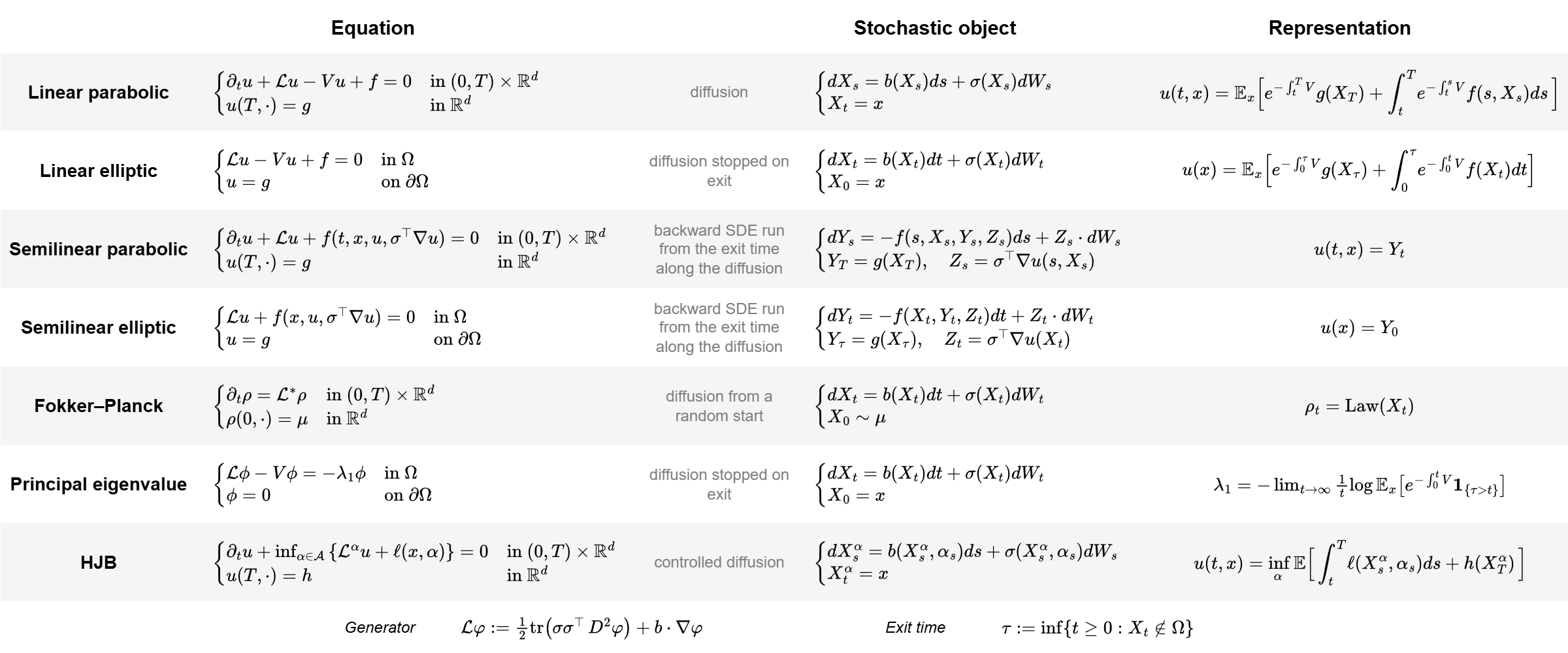

4.1 Boundary conditions

Name	PDE ingredient	Stochastic object
Dirichlet condition	$u=g$ on $\partial\Omega$	process killed on contact
Neumann condition	$\partial_n u=0$	reflected diffusion
Robin condition	$\partial_n u=\alpha u$	reflected diffusion killed at rate $\alpha$ in local time

4.2 Other families

So far we have only considered stochastic processes driven by Brownian motion, but the Feynman–Kac theorem is more general.

A finite state space

Let $\xi$ be a continuous-time Markov chain on $\{1,\dots,n\}$ with generator matrix $Q$ and let $V\in\mathbb{R}^n$ be a killing rate. The “PDE” is then a linear system of ODEs,

$$ u'(t) \;=\; \big(Q-\operatorname{diag}V\big)\,u(t), \qquad u(0)=g\in\mathbb{R}^n , $$

and the Feynman–Kac formula reads

$$ u_i(t)\;=\;\mathbb{E}_i\Big[e^{-\int_0^t V(\xi_s)\,ds}\,g(\xi_t)\Big], \qquad\text{that is}\qquad u(t)=e^{t(Q-\operatorname{diag}V)}\,g . $$

The generator has replaced the Laplacian and a matrix exponential has replaced the heat semigroup; not a single other word of the argument changes. It is a useful version to keep in mind, because it makes plain that the theorem is a statement about generators and semigroups, and not about Brownian motion.

Lévy processes

Replace $W$ by a Lévy process. The simplest case is a compound Poisson path that waits an exponential time of rate $\lambda$ and then jumps,

$$ X_t \;=\; x+\sum_{i=1}^{N_t}Z_i , $$

with $N_t$ a Poisson process of rate $\lambda$, the $Z_i$ independent draws from a distribution $\mu$. Its generator is an integral operator, and the equation becomes

$$ \begin{cases} \partial_t u(t,x) = \lambda\!\int\big[u(t,x+z)-u(t,x)\big]\,\mu(dz)\;-\;V(x)\,u(t,x),\\ u(0,\cdot)=g, \end{cases} $$

while the representation remains unchanged:

$$ u(t,x)=\mathbb{E}_x\big[e^{-\int_0^tV(X_s)ds}g(X_t)\big]. $$

What is new is that the operator is nonlocal: the value at $x$ is tied to the value at every $x+z$ the path can reach in one jump, not merely to an infinitesimal neighbourhood.

Letting the jump measure be $\nu(dz)=c_{d,\alpha}|z|^{-d-\alpha}dz$ makes $X$ an $\alpha$-stable process and $\mathcal{L}=-(-\Delta)^{\alpha/2}$, so the fractional heat equation is Feynman–Kac for a pure-jump path. Nonlocality does cost something at the boundary: a jump can leave $\Omega$ without ever touching $\partial\Omega$, so a Dirichlet datum must be prescribed on the whole complement $\Omega^c$.

Mean field games

Let the cost of one player depend on where everybody else is. Against a given flow of population densities $(m_s)_{s\le T}$, a representative player steers

$$ dX_s \;=\; \alpha_s\,ds+\sigma(X_s)\,dW_s ,\qquad X_0\sim m_0 , $$

and the value of their problem is a Feynman–Kac representation, now with an optimization in front of the expectation,

$$ u(t,x)\;=\;\inf_{\alpha}\;\mathbb{E}\Big[\int_t^T\big(L(X_s,\alpha_s)+F(X_s,m_s)\big)ds+G(X_T,m_T)\;\Big\vert\;X_t=x\Big]. $$

Writing $H(x,p)=\sup_{\alpha}\{-\alpha\cdot p-L(x,\alpha)\}$ for the Hamiltonian, that infimum is attained at the feedback $\alpha^{*}=-\partial_pH(x,\nabla u)$, and equilibrium demands that the flow the player generates by using it be the flow they were given, $m_s=\operatorname{Law}(X_s)$. The two requirements together are a forward–backward system,

$$ \begin{cases} -\partial_t u-\mathcal{L}u+H(x,\nabla u)=F(x,m_t), & u(T,\cdot)=G(\cdot,m_T),\\[4pt] \ \ \partial_t m-\mathcal{L}^{*}m-\operatorname{div}\big(m\,\partial_pH(x,\nabla u)\big)=0, & m_0\ \text{given}, \end{cases} $$

in which the backward Hamilton–Jacobi–Bellman equation is the value of a representative player and the forward Fokker–Planck equation transports the population density under the feedback $-\partial_pH(x,\nabla u)$ that the first equation produces. The two are coupled through $m$: the cost a player faces depends on the distribution of all players, and that distribution is the law of the very process the player is optimizing. So the object to solve for is a fixed point in a space of flows of measures, and the equations run in both time directions at once. It is the $N\to\infty$ limit of a Nash equilibrium among $N$ symmetric players.

Both halves can be carried by a single path. Along the optimally controlled process, with $Y_s=u(s,X_s)$ and $Z_s=\sigma^\top\nabla u(s,X_s)$, the system becomes one probabilistic object, a McKean–Vlasov forward–backward SDE:

$$ \begin{cases} dX_s=-\partial_pH\big(X_s,\sigma^{-\top}Z_s\big)ds+\sigma(X_s)\,dW_s, & X_0\sim m_0,\quad m_s=\operatorname{Law}(X_s),\\[4pt] dY_s=-\big[L(X_s,\alpha^{*}_s)+F(X_s,m_s)\big]ds+Z_s^\top dW_s, & Y_T=G(X_T,m_T). \end{cases} $$

The forward line is the path that uses the optimal feedback and whose law is the population itself; the backward line carries the cost still to be paid, and its martingale part $Z$ is again $\sigma^\top\nabla u$, the hedging portfolio of the linear theory. What is genuinely new is that the coefficients depend on $\operatorname{Law}(X_s)$, so the expectation is taken under a measure the equation itself has to produce. This is the nonlinear Feynman–Kac of Pardoux–Peng [5]: the conditional expectation of the linear theory becomes a backward SDE, and the fixed point in flows of measures is what the forward–backward coupling means in probabilistic terms.

References

[1] R. P. Feynman. Space-Time Approach to Non-Relativistic Quantum Mechanics. Reviews of Modern Physics 20 (1948) 367–387.

[2] M. Kac. On Distributions of Certain Wiener Functionals. Transactions of the American Mathematical Society 65 (1949) 1–13.

[3] F. Black and M. Scholes. The Pricing of Options and Corporate Liabilities. Journal of Political Economy 81 (1973) 637–654.

[4] I. Karatzas and S. Shreve. Brownian Motion and Stochastic Calculus. 2nd ed., Springer, 1991. (§4.2–4.4 for the Dirichlet problem, §5.7 for Feynman–Kac.)

[5] E. Pardoux and S. Peng. Adapted solution of a backward stochastic differential equation. Systems & Control Letters 14 (1990) 55–61.

[6] J.-M. Lasry and P.-L. Lions. Mean field games. Japanese Journal of Mathematics 2 (2007) 229–260.